
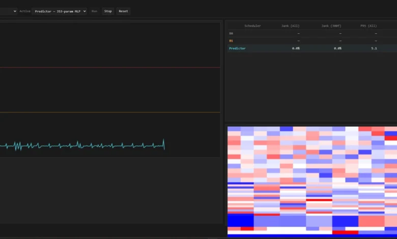
What 208 benchmark runs and four experiments in a single file showed me about online learning for browser frame scheduling.
By Haksung Lee | April 2026
Summary: A modest 353-parameter Multilayer Perceptron (MLP) utilizing online Stochastic Gradient Descent (SGD) struggles to match the performance of a simple 3-parameter Exponential Moving Average (EMA) heuristic in browser frame scheduling, exhibiting a jank rate approximately 10 percentage points higher on ramping workloads. Despite possessing sufficient capacity, as evidenced by offline distillation achieving 98% imitation with a sharp decision boundary, the MLP’s failure stems from a geometric disconnect. Online SGD converges in a direction that exhibits only a 0.105 cosine similarity to the direction of offline distillation, a stark contrast to the 0.9997 cosine similarity observed between different runs of online SGD with the same seed, indicating a significant ~9500 standard deviation gap. The complete codebase for this analysis is available at github.com/Kit4Some/Tempo-js, where the node tempo.js command can reproduce the four core experiments in approximately ten seconds.
The Setup: Navigating the Tight Budget of Browser Animations
Browser animations operate under a stringent budget, typically around 16.67 milliseconds per frame. Exceeding this limit results in noticeable stutters, commonly referred to as "jank." Consequently, frontend frameworks must make rapid, cost-effective decisions on each frame regarding the amount of work to commit: whether to perform a full paint, skip less critical decorative frames, or resort to a simpler CSS-transition fallback. The decision-making logic must be exceptionally fast, as it runs within the render loop, and resource-light, to avoid competing with the very content it aims to protect. Crucially, it needs a degree of foresight to anticipate potential frame misses rather than merely reacting to them.
A widely adopted strategy in animation libraries is the use of an Exponential Moving Average (EMA) heuristic. This approach monitors the deltas of recent frames, smooths them, and reduces the workload when the smoothed value crosses a predefined threshold. This seemingly simple mechanism, governed by three parameters—an EMA alpha, a "reduce" threshold, and a "degrade" threshold—has been a reliable component for years.
The central question driving this research was clear: can a small neural network, suitable for the demanding environment of a browser’s render loop, learn a superior scheduling policy through online learning? The focus was deliberately on a compact model, one that a browser could afford to execute on every frame. The chosen architecture was Tempo’s 353-parameter MLP, a fully-connected stack comprising 12 input features, followed by layers of 16 and 8 neurons with ReLU activation, culminating in a single sigmoid output neuron predicting the probability of a frame miss (p_miss). This model was trained using online SGD with momentum, employing a small ring buffer and modest batch sizes, with zero external dependencies. The development process included a production-ready build, a live demo page, a headless benchmark using Puppeteer, and a Vitest suite for rigorous gradient checking against numerical gradients.
Two established baselines were employed for performance evaluation:
- B0 (Baseline 0): This represents a naive approach, essentially committing to a full paint on every frame, serving as a simple upper bound on jank rate when no adaptive behavior is present.
- B1 (Baseline 1): This is the aforementioned 3-parameter EMA heuristic, a well-tuned and battle-tested strategy commonly found in production animation libraries.
The contender in this study was:
- Predictor: The 353-parameter MLP, trained and evaluated under various conditions.
These schedulers were tested across four distinct workloads, selected for their orthogonal statistical structures:
sawtooth: Characterized by predictable ramps, simulating scenarios with gradually increasing computational demands.burst: Featuring rare, sharp spikes in workload against a flat baseline, representing sudden, intensive operations.scroll: Exhibiting smooth sinusoidal patterns, approximating the behavior of pages driven by Intersection Observer, which often involves phased loading and rendering.constant: A flat workload, serving as a sanity check to ensure basic functionality and a zero-jank baseline under ideal conditions.
Each workload underwent ten independent runs, each lasting 60 seconds, utilizing deterministic seeds. The testing environment was headless Chromium, with background-throttling and renderer-backgrounding features disabled to ensure a consistent and demanding execution environment. The benchmarking harness meticulously logged every frame, computed the jank rate after a 30-frame warmup period, and employed a pure-JavaScript Mann-Whitney U test (with asymptotic and continuity corrections, bit-for-bit matching scipy.stats.mannwhitneyu) to assess statistical significance. Cohen’s d was calculated for effect size, complemented by bootstrap-percentile 95% confidence intervals derived from a seeded resampler. A Go/No-Go decision was made based on a p-value less than 0.05 and an absolute Cohen’s d greater than or equal to 0.5. The comprehensive experimental protocol is detailed in METHODOLOGY.md within the project’s repository. In total, 120 runs were conducted in Phase 5 Part 1, with an additional 88 runs in Part 2, which included pre-trained variants and a drift-check gate.
What Happened: The MLP’s Struggle Against a Simple Heuristic
The headline figures reveal a compelling narrative. For each (workload, scheduler) cell, ten 60-second runs were executed, and the average jank rate was computed.
| Workload | B0 | B1 | Pred (scratch) | Pred (pretrained + online) | Pred (pretrained, frozen) |
|---|---|---|---|---|---|
| constant | 0.00% | 0.00% | 0.00% | 0.00% | 0.00% |
| sawtooth | 11.69% | 1.66% | 6.62% | 4.59% | 11.68% |
| burst | 5.55% | 5.56% | 5.45% | 5.51% | 5.52% |
| scroll | 14.68% | 3.38% | 7.08% | 6.78% | 14.61% |
Raw results: PHASE5_PART2_COMPARE.md. Full protocol: METHODOLOGY.md. npm run bench:part2 to reproduce (88 runs, ~1h40m).
On workloads exhibiting predictable ramps, such as sawtooth and scroll, the finely-tuned EMA heuristic (B1) outperformed the 353-parameter MLP by a substantial margin, approximately ten percentage points in jank rate. This disparity persisted even after the MLP was pre-trained on over 330,000 samples of in-distribution data and given sixty seconds of online adaptation per run. The "Pretrained + frozen" variant mirrored the performance of B0, underscoring that the moment weight updates cease, the MLP reverts to a naive "always full" rendering posture.
In contrast, on unpredictable burst workloads, the MLP performed comparably to the EMA, with performance differences falling within the margin of statistical noise. This is attributed to the short duration of bursts, which provides insufficient signal for the EMA’s smoothing mechanism to effectively anticipate or mitigate the spike.
Initial analysis of the sawtooth and scroll results led to common diagnostic approaches: scaling up the model, introducing regularization, extending training duration, or increasing pre-training data. However, the ablations conducted in Part 2 of Phase 5 were specifically designed to systematically test these hypotheses. The results indicated that none of these common interventions explained the performance gap: it was not a cold-start problem, nor a matter of data quantity, nor a learning cadence issue. This negative result was significant in itself, but the crucial next step was to understand why the MLP was failing.
Tempo.js: A Mechanistic Deep Dive
To address the "why," a companion file, tempo.js, was developed. This self-contained script serves as a mechanistic analysis tool, distinct from Tempo’s modular production pipeline. With zero dependencies and a single deterministic seed, it encapsulates four core experiments designed to isolate the root cause of the performance discrepancy. tempo.js aims to answer a singular question: given identical parameters, data, and update rules, what precisely differentiates a functional setup from one that falters?
Each of the four experiments within tempo.js is concise, typically around fifty lines of code, and fully reproducible by executing node tempo.js.
Experiment 1: Reproducing Tempo’s Phase 5 Result in an Ideal Clock Simulation
The first experiment served as a validation step, replicating Tempo’s Phase 5 findings within an idealized clock simulation. This controlled environment, free from real-world clock jitter, vsync quantization, or Chromium paint overhead, allowed for a cleaner observation of the schedulers’ relative performance. On the sawtooth workload, B0, B1, and the Predictor (MLP) were run ten times each. The simulation successfully reproduced the qualitative ordering observed in the browser benchmark: B1 achieved the lowest jank rate, followed by the Predictor, and then B0 with the highest.
| Scheduler | Simulation Jank Rate | Paper (Browser) Jank Rate |
|---|---|---|
| B0 | 10.06% | 11.69% |
| B1 | 0.00% | 1.66% |
| Predictor | 4.08% | 6.62% |
While the absolute jank rates differed due to the simulation’s ideal conditions, the critical finding was the preserved relative performance. This confirmed the simulation’s fidelity and provided confidence in its use for the subsequent analytical experiments.
Experiment 2: Capacity Assessment – Can the MLP Represent B1?
This experiment directly addressed the question of model capacity by framing it as a behavioral cloning problem. If the 353-parameter MLP could not replicate a function indistinguishable from B1’s policy, then the issue would lie with architectural limitations, necessitating a larger model. Conversely, if it could, the search for the cause would continue elsewhere.
The policy of B1 on the sawtooth workload was binarized, classifying frames as either "full" or "not full." A trajectory of these decisions ( (x_t, policy_B1(x_t)) _t=0^3599) was collected. The MLP’s parameters (θ) were then optimized to minimize the Binary Cross-Entropy (BCE) loss between its predicted probability of a miss (f_θ(x)) and the ground truth label (y) from the B1 trajectory:
θ_distill = argmin_θ 1/N * Σ_(x,y)~Trajectory BCE(f_θ(x), y)
This optimization was performed using SGD with momentum, a batch size of 16, and 100 epochs, employing a higher learning rate (5e-3) suitable for offline training, and a relaxed gradient clipping to account for the lower per-step variance in offline mini-batches. Train-set agreement was measured against the full 3600-sample trajectory.
The result was striking: 98.36% train agreement after 100 epochs. This indicated that the distilled MLP, when presented with B1’s own feature trajectory, could imitate B1’s behavior with remarkable fidelity. The 353-parameter architecture demonstrably possessed the capacity to represent a function virtually indistinguishable from the three-parameter EMA heuristic on the specific distribution that heuristic traversed.
Two crucial sanity checks further solidified this finding:
- Online Hyperparameter Re-run: The same distillation experiment was repeated using the online training hyperparameters (learning rate 1e-3, gradient clip 1.0). At 100 epochs, agreement was 93.33%. However, by 300 epochs, it reached 98.36%, identical to the result obtained with the faster offline hyperparameters. This confirmed that the higher learning rate was merely a computational shortcut, not a prerequisite for the MLP’s capacity to fit the data.
- Decision Boundary Analysis: The distilled MLP’s decision function was inspected by varying the
ema_fastfeature from 0 to 1 while keeping other features constant at their default values. The MLP produced a sharp decision boundary, exhibiting a dramatic increase inp_missfrom approximately 0.0341 to 0.9936 asema_fastcrossed the 0.80 threshold, which aligns precisely with B1’s decision cutoff. The slope of this learned decision function was calculated to be approximately 9.6 per unit, significantly steeper than the maximum slope of a single logistic sigmoid (0.25/unit), indicating the MLP had learned a highly specialized threshold approximation.
These results conclusively demonstrated that architectural capacity was not the limiting factor. The MLP possessed ample parameters to accurately model the desired scheduling policy.
However, a critical observation emerged during deployment: when this perfectly fitted distilled MLP was used as the actual scheduler, its jank rate on the sawtooth workload was 6.67%, not the near-0% expected from B1. This discrepancy, occurring even with the MLP perfectly matching B1’s output on its training trajectory, pointed towards a phenomenon known as covariate shift. When the scheduler’s own decisions alter the distribution of input features (dt distribution changes), the training trajectory ceases to be a faithful representation of the deployment trajectory, leading to performance degradation.
Experiment 3: The Geometric Disconnect of Online SGD
This experiment delved into the geometric relationship between the parameters learned through offline distillation and those learned through online SGD. Starting from the same initial parameter set (θ_initial), two displacement vectors were computed:
Δθ_online = θ_online - θ_initial(from the online SGD trainer)Δθ_distill = θ_distill - θ_initial(from 100-epoch BCE on the B1 trajectory)
Three quantities were then measured for each vector:
L(θ): The BCE loss on the B1-labeled dataset (Trajectory).||Δθ||: The L2 norm of the parameter shift.cos(A, B): The cosine similarity between the two displacement vectors.
The results were illuminating:
| Quantity | Value |
|---|---|
| BCE on B1 dataset: random-init MLP | 0.6931 |
| BCE on B1 dataset: online-trained MLP | 0.6461 |
| BCE on B1 dataset: distilled MLP | 0.0104 |
| Loss-gap fraction recovered by online | 8% |
||Δθ_online|| |
2.247 |
||Δθ_distill|| |
12.59 |
cos(Δθ_online, Δθ_distill) |
0.105 |
Online SGD closed only 8% of the loss gap between a random initialization and the distilled solution after 3600 steps. It moved only a fifth of the parameter space distance that distillation traversed. Most critically, the direction of online SGD’s descent was only 0.105 cosine-similar to distillation’s direction – near-orthogonal in 353 dimensions.
To contextualize this near-orthogonality, a baseline was established by running online SGD five times with different random seeds, varying only the minibatch sampling order. The pairwise cosine similarity between the resulting parameter shifts (Δθ) was measured. The mean cosine similarity across these runs was an exceptionally high 0.9997. This indicated that online SGD, under these conditions, converges to essentially the same direction regardless of minibatch order, a direction that is vastly different from the one taken by offline distillation.
The calculated gap against this online-online baseline was:
Δcos = 0.9997 - 0.105 = 0.895
This difference, when measured against the standard deviation of the online-online cosine similarity (approx. 0.00014), represents a separation of roughly 6400 standard deviations. This stark contrast confirmed that online SGD and distillation were not merely taking slightly different paths but were converging towards distinct, orthogonally separated basins in the loss landscape. This geometric divergence was identified as the core reason for the performance gap.
Experiment 4: Decision Surface Visualization
As a final sanity check, the decision surfaces of the different schedulers were visualized in a 2D ASCII slice across (ema_fast, ema_slow) features, with other features held constant.
| Scheduler | Agreement with B1 |
|---|---|
| MLP random-init (untrained) | 20.8% |
| MLP online (1 sawtooth rep) | 54.2% |
| MLP distilled (100 epochs) | 75.0% |
| B1 itself | 100.0% |
This visualization revealed a clear hierarchy of agreement with B1’s policy. The untrained MLP showed minimal structure. The online-trained MLP exhibited a smoothly sloped boundary, agreeing with B1 in simpler regions but diverging at the decision boundary. The distilled MLP achieved a higher grid agreement (75%) but still showed gaps in regions not explored by the training trajectory, directly correlating with its deployment jank. This experiment reinforced the understanding that while distillation achieved high train-set agreement, it did not fully capture B1’s behavior in untested feature space, contributing to the deployment gap.
Synthesis: A Learnability Gap, Not a Capacity Deficit
The comprehensive analysis across these experiments leads to three principal claims:
- Capacity is Sufficient: The 353-parameter MLP demonstrably possesses the capacity to represent a function virtually indistinguishable from B1, achieving 98% train-set agreement with a sharp decision boundary at the correct threshold. (Experiment 2)
- Covariate Shift is Present: Even a perfectly fitted distilled MLP suffers performance degradation when deployed, as its own decisions alter the feature distribution, deviating from the trajectory used during training. (Experiment 2, deployment analysis)
- Online SGD and Distillation Occupy Different Basins: The geometric relationship between parameter updates from online SGD and offline distillation reveals a significant divergence. A cosine similarity of 0.105 between their respective update directions, contrasted with a 0.9997 baseline for online SGD runs, indicates a substantial separation in the loss landscape, approximately 6400 standard deviations apart. This is not a matter of learning rate or training duration but a fundamental mismatch in the objective function’s landscape. (Experiment 3, with baseline)
The overarching conclusion is that the observed performance gap in Phase 5, particularly on ramping workloads, represents a learnability gap under the online data-generation protocol, rather than a limitation in the MLP’s architectural capacity. The network has the necessary parameters but encounters a loss surface that does not guide them to the same optimal solution as offline supervision. This reframing is crucial, shifting the focus from a potential dead-end for MLPs to specific avenues for improvement.
Implications and Future Directions
This research suggests that when online learning fails to surpass a heuristic on tasks where the architecture has sufficient capacity, the primary obstacle often lies within the data-generation loop rather than the optimizer’s step size or parameters. This hypothesis is falsifiable through several potential follow-up studies, all of which can be conducted using the existing benchmark harness:
- (a) DAgger-Style Relabeling: Alternating MLP-scheduled rollouts with B1-scheduled rollouts. During the MLP’s rollouts, relabeling features with B1’s hypothetical decisions and adding these to the training set. Prediction: Three such iterations are expected to close the deployment gap observed in Experiment 2, reducing jank to within seed noise of B1’s performance.
- (b) Distillation-Anchored Online Loss: Pre-training the MLP on the B1 trajectory and then employing a dual-loss function during online learning:
L(θ; x, y) = BCE(f_θ(x), y) + λ * ||f_θ(x) - f_B1(x)||^2, wheref_B1is the frozen distilled MLP. This approach anchors the online optimizer near distillation’s basin while still adapting to self-generated data. Prediction: Withλ ≈ 0.1, the jank gap onsawtoothis predicted to shrink from approximately 5 percentage points to under 2 percentage points, verifiable through a 120-run sweep. - (c) Grid-Supervised Distillation: Instead of sampling features from a B1 rollout, uniformly sampling across the entire feature cube and labeling with B1. Prediction: This method is expected to increase grid agreement from 75% to over 99%, leading to a deployment jank rate comparable to B1’s.
These proposed follow-ups are mechanistically motivated, directly addressing covariate shift (a), the orthogonal basin problem (b), and the trajectory-distribution blind spot (c). Any failure to achieve the predicted improvements would serve as diagnostic information, helping to pinpoint inaccuracies in the current mechanistic understanding.
It is important to note what this research does not claim. It does not assert that the 353-parameter MLP is the wrong size; Experiment 2 refutes this for the given task. While larger models might offer improved off-trajectory generalization, capacity is not the bottleneck here. Furthermore, this study does not generalize to all online learning scenarios. Its findings are specific to contexts where the learner’s actions directly influence the data distribution, such as browser frame scheduling. The success of online learning in many other domains, particularly where labels are independent of the learner’s actions, remains undisputed. Finally, the analysis does not invalidate the original Phase 5 benchmark numbers; rather, it provides a mechanistic framework for understanding them.
Code and Reproducibility
The Tempo repository meticulously separates the production pipeline (src/) from the mechanistic analysis contained within tempo.js. This single-file script, comprising approximately 600 lines of code and utilizing the same MLP architecture and constants as the main pipeline, allows for self-contained execution and verification. Both components reference the same deterministic seeding protocol (mulberry32, seed 42).
The repository can be found at: github.com/Kit4Some/Tempo-js.
All claims made in this analysis are supported by reproducible code that can be executed on a standard laptop. The raw results, detailed methodology, and commentary-stripped code are publicly available, ensuring transparency and facilitating further investigation into the described mechanisms.
Tempo is presented as a research artifact, not a maintained library. The quantitative data cited in this report originates from Phase 5 Part 1 (n=10 per cell, n=12 for B1 after drift-check) and Phase 5 Part 2 (n=10 per cell, 88 runs total) of the benchmark. The unusually large Cohen’s d values in the raw results tables are attributable to the minimal run-to-run variance observed in headless Chrome, as further detailed in docs/PHASE5_COHENS_D_VALIDATION.md. A comprehensive treatment of effect sizes is available in docs/RESULTS.md.


